Vlookup Multiple Criteria Tutorial in Excel 2013

Udemy Editor

Excel is a powerful way of creating, storing and analyzing lists of data for business purposes. The functions in Excel allow you to sort and retrieve data from large spreadsheets using formulas like the Lookup formulas in Excel. Learning to use the Vlookup or Lookup formula can save you time where you need to find specific data based on certain criteria. This tutorial will show you how to use the CONCATENATE formula to useVlookup to search multiple criteria within your data. This tutorial assumes you know how to create a spreadsheet and that you know how to work with formulas and functions in Excel.

Microsoft Excel 2013 Simplified will teach you the basics of Excel and how to work with the various elements within Excel. This course offers 110 lectures to help you learn to harness the power of Excel at the office and at home. The course is aimed at introducing beginners to the program and also helping more advanced users to improve their Excel skills. You will learn how to create worksheets and the course will slowly take you through the functions of Excel until you are able to handle advanced topics with ease.

Understanding the Vlookup Function

The Vlookup function is designed to help you look up specific data in a list or array of data based on a specific criteria that you set. The Vlookup function is built to find data based on one column of data, but Vlookup can be used in conjunction with other functions to allow you to search using Vlookup based on multiple criteria. Using one function within another function is called nesting functions and the real power of Excel lies within its power to nest the functions you can use.

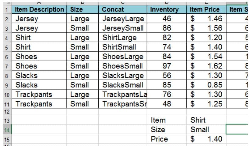
The following example will show you how to use two criteria in the Vlookup function using the concatenate function. The tutorial is based on the following example data:

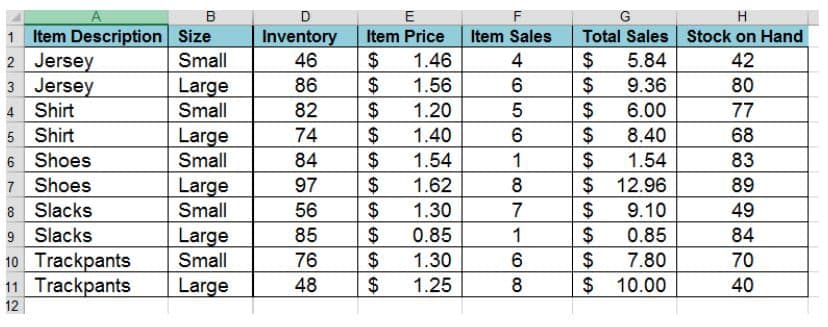
We are going to create a function to search for the price of a specific item and item size. The Vlookup function requires a unique field to find. As you can see from the example we have two rows for each item, one for the small size and one for the large size. So we first need to use the concatenate function to create a unique field to search on before we use the Vlookup function.

To learn how to use the various functions in Excel, sign up for the Excel 2013 course now and learn to use Excel like a master. This course contains 101 lessons that will introduce you to Excel 2013 and will teach you the basics and more advanced concepts in Excel.

Concatenate to Create Unique Identifier

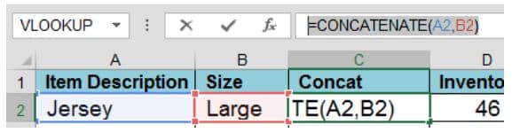
So we will first create a new column to create a unique identifier for our search. Add a column to your worksheet and then CONCATENATE the “Item” and “Size” fields to create a new unique identifier:

This is the formula you will need to use to create the new column:

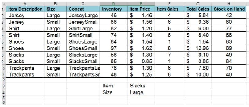
Now that we have a unique identifier, we can create two input fields for our search. Add a new cell called Item and one called Size so that spreadsheet users can enter the item and size they are looking for:

Now add a field for Price and then we will add the Vlookup formula to lookup the price of the item.

Adding the Vlookup Formula

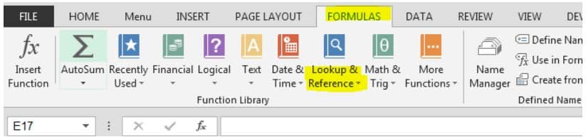
We are going to use the formula wizard to add the Vlookup formula for our spreadsheet. To start the formula wizard, select the “vlookup” formula from the “Lookup & Reference” Formulas under the Formulas Tab:

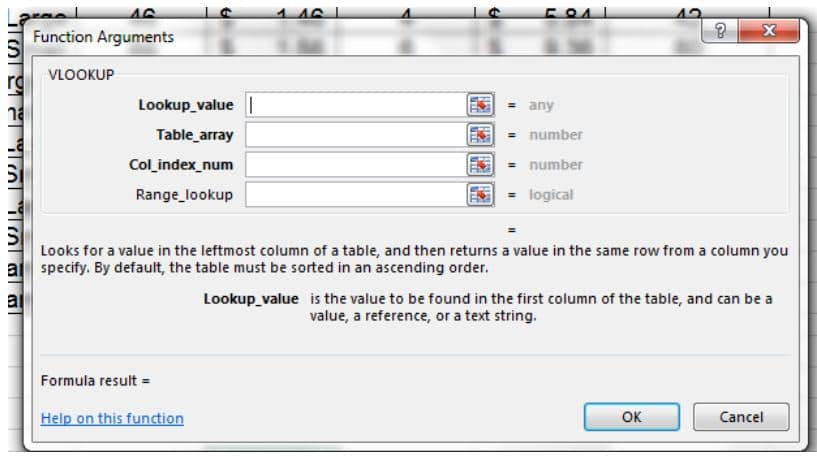
The following formula wizard will open up:

Enroll in the Excel 2013 The Basics course now and learn to use the formulas and functions available in Excel. This course offers 160 lessons and downloadable worksheets to help you learn all the Excel skills you need to master Excel 2013. The course will get you started with Excel, it will teach you how to perform calculations, how to modify a worksheet, how to format the worksheet and how to save. You will learn to manage large workbooks; it will teach you Excel formulas to make you life easier and you can follow along in the downloadable workbooks.

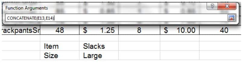
Add the Lookup Value

We now need to tell Excel what we are looking for in the Vlookup wizard. Remember we have created a new column that represents the concatenation of the item name and item size. So we need to find the concatenation of the item and size when we search for the data. To add the concatenation formula to our wizard, click the formula and then type in CONCATENATE(E13,E14) to create a field that will match our list based on what a user types in under item and item size:

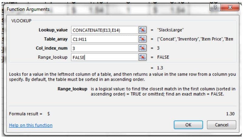
The table we want to search must start with the column that contains the field we are looking for, so the table we are searching for is C1:H11. The column we want to search for the answer – in this case we are searching for the price of the item – is column number 3 because column number 3 is the 3rd column in the table we are searching. Finally we will enter FALSE because we are looking for an exact match for our search and not the closest match.

You completed formula wizard will look like this:

If a user types in “Shirt” and “Small” The answer will look like this:

Multiple String Search Criteria

Concatenate is a great way to use multiple search criteria when the criteria are all strings. You can concatenate as many fields as you like using the concatenate function so you can create a unique field and then use the same concatenation to create a unique value to search those fields.

Join thousands of students who have enrolled in Excel 2013 For Dummies Video Training, Deluxe Edition to harness the power of Excel in their homes and their working lives.

For more tutorials on the lookup function read: