How to Use VLOOKUP in Excel: A Step-by-Step Guide

If you’ve ever found yourself scrolling endlessly through thousands of rows in Excel, squinting at your screen to match a product SKU with its price, I have some great news for you: You don’t have to do that anymore. In the world of spreadsheets, there is life before learning VLOOKUP, and life after.

VLOOKUP is the ultimate gateway from Excel basics to advanced Excel proficiency. Whether you are managing inventory for a local surf shop, sorting through employee records, or pulling sales data for a quarterly review, mastering this function will save you hours of manual work and make you look like an absolute wizard to your boss.

In this comprehensive, step-by-step guide, we are going to break down VLOOKUP together. No complicated jargon—just clear, practical examples, visual guides, and battle-tested troubleshooting tips. 

What is VLOOKUP? (And Why You Need It)

In Excel, VLOOKUP stands for Vertical Lookup.

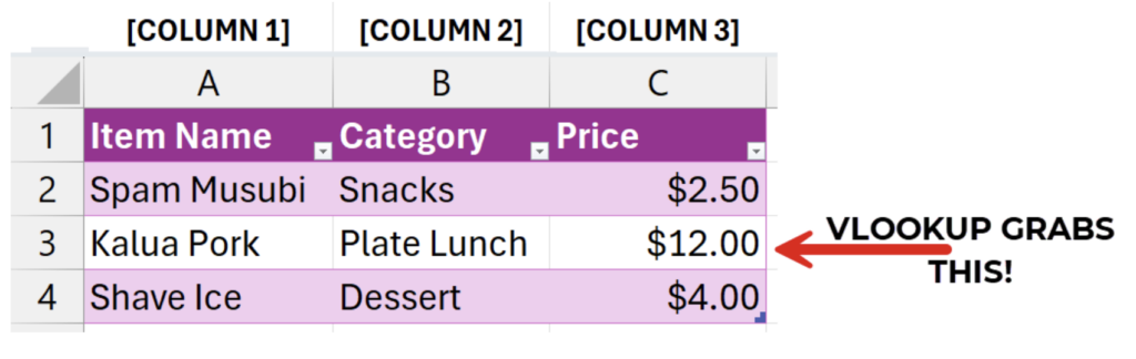
Think of it like looking at a menu at your favorite plate-lunch spot. If you want to know how much a “Kalua Pork” plate costs, your eyes naturally do two things:

1. They scan vertically down the first column (the list of food items) until they locate “Kalua Pork.”
2. They look horizontally to the right to find the price in the next column.

That is exactly what VLOOKUP does. It searches vertically down the very first column of a selected table to find a specific value. Once it finds that value, it travels across that row to a column you specify and pulls back the corresponding piece of data.

VLOOKUP vs. HLOOKUP

While VLOOKUP searches columns vertically, HLOOKUP (Horizontal Lookup) searches rows horizontally. Because 99% of professional databases and spreadsheets are organized vertically with column headers, VLOOKUP is the tool you will use almost every day.

Deciphering the VLOOKUP Formula Syntax

Before we start writing, let’s look at the blueprint. If you type VLOOKUP manually into a cell, this is the syntax Excel expects:

=VLOOKUP(lookup_value, table_array, col_index_num, [range_lookup])

Don’t let the technical terms scare you. Let’s break down these four arguments into plain English:

Argument	What it means in plain English	Practical Example
lookup_value	What do you want to find? (The starting search term).	“Kalua Pork” or cell A3
table_array	Where is the search grid? (The range containing your data).	A2:C4
col_index_num	Which column holds the answer? (Counted from left to right, starting at 1).	3 (for Price in Column C)
range_lookup	Do you want an Exact match or an Approximate match?	FALSE (Exact) or TRUE (Approximate)

🤙 Billy’s Masterclass Note #1: The Golden Rule of VLOOKUP

The most critical rule of VLOOKUP is that your lookup_value MUST reside in the very first (leftmost) column of your table_array. If you want to search by Employee ID, then Employee ID must be in Column 1 of the range you select. VLOOKUP cannot look to its left! If your data isn't set up this way, you'll run into a wall. (More on how to handle this later!)

The Anatomy of the Arguments

Let’s dig a little deeper into how these elements work so you can write formulas confidently without relying on guesswork.

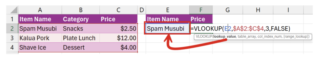
1. The Lookup Value (lookup_value)

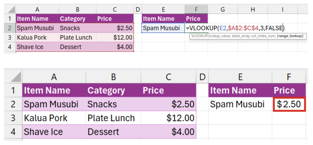
This is your starting point. It can be text inside quotation marks (like “Spam Musubi”) or, more commonly, a dynamic cell reference (like E2).

Using cell references is highly recommended because it allows your formula to update automatically when you change the value in that cell.

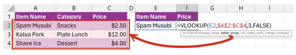
2. The Table Array (table_array)

This is the block of data Excel will search. It should encompass both your search column and the column containing the answer you want to find.

📌 Pro-Tip: Lock Your Ranges!

When you write a VLOOKUP formula and drag it down to apply it to other rows, Excel’s relative cell references will shift downwards too (A2:C4 becomes A3:C5, then A4:C6). This is called “range shifting,” and it will cause your lookup to break!

To prevent this, always lock your table array using absolute references by adding dollar signs ($).

• Standard reference: A2:C4 (Will shift when copied)
• Absolute reference: $A$1:$C$4 (Locked in place!)
• 🤙Billy’s Shortcut: Highlight your table array in the formula bar and press the F4 key (or Cmd + T on a Mac) to apply dollar signs instantly.

3. The Column Index Number (col_index_num)

This tells Excel which column to pull the data from. You must provide this as a number, counting from left to right, beginning with your search column as 1.

• Column 1 = The search column
• Column 2 = The next column to the right
• Column 3 = The third column… and so on.

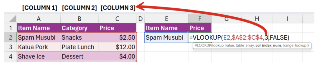
If you want to return the Price, your col_index_num is 3.

4. Exact vs. Approximate Match (range_lookup)

This is the final, optional argument, but do not ignore it! Leaving it blank is the #1 mistake Excel beginners make.

• FALSE (or 0): Exact Match. This tells Excel, “Find me exactly what I asked for, or return an error.” You will use this 95% of the time (e.g., searching for product names, employee IDs, serial numbers).
• TRUE (or 1): Approximate Match. This tells Excel to look for the closest value that is less than or equal to your lookup value. This is used for ranges, like tax brackets, grading scales, or shipping rate tiers. Crucial rule: Your first column must be sorted in ascending order for TRUE to work properly.

⚠️ Fact-Check Warning: If you leave this argument blank, Excel defaults to TRUE. If your data is unsorted, this will return incorrect, unpredictable data. Always type FALSE to play it safe!

Step-by-Step Walkthrough: VLOOKUP in Action

Let’s run through a practical, real-world scenario. Imagine we manage a tropical fruit wholesale business and have the following master inventory table:

Our Master Dataset (Sheet Name: “Inventory”)

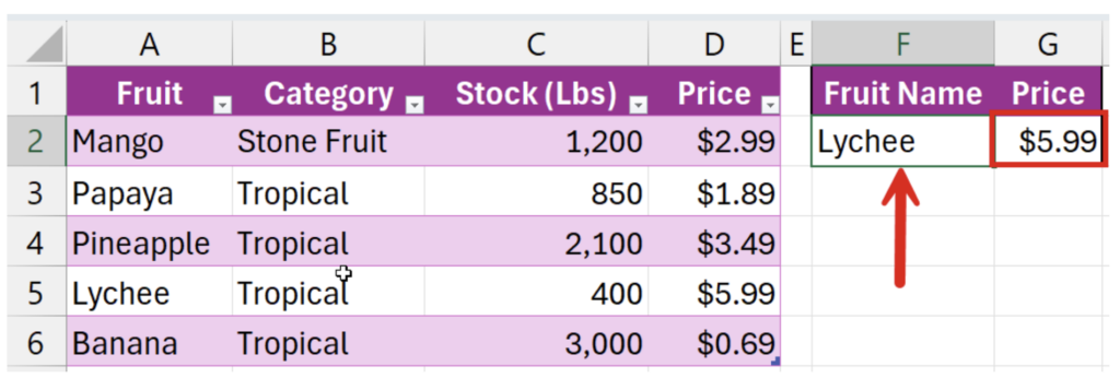
We want to build a dynamic “Price Lookup Tool” in cell G2. When we type a fruit name into cell F2, we want VLOOKUP to instantly fetch the correct price from our dataset.

Option A: The Manual Method (Fastest)

If you are comfortable typing formulas directly, here is how you write it:

1. Click on cell G2.
2. Type =VLOOKUP( to begin.
3. Select cell F2 (our lookup_value). This is the cell where we’ll type our fruit name. Type a comma.
4. Select our table range. Since our search value is “Fruit” (Column A) and the target value is “Price” (Column D), our table array must start at Column A. Let’s select range A2:D6. Lock it by pressing F4 so it becomes $A$2:$D$6. Type a comma.
5. Count the columns starting from “Fruit” (Column A) to “Price” (Column D):

• Fruit (Col A) is 1
• Category (Col B) is 2
• Stock (Col C) is 3
• Price (Col D) is 4 So, enter 4 as your col_index_num. Type a comma.

6. Type FALSE to ensure we get an exact price match.
7. Close the parentheses and press Enter.

Your completed formula looks like this:

=VLOOKUP(F2, $A$2:$D$6, 4, FALSE)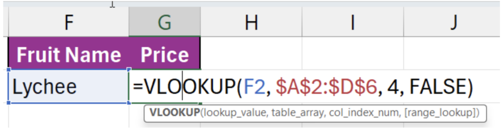

Option B: Using the Excel Formula Builder (Great for Beginners)

If you don’t want to type the formula manually, you can use Excel’s built-in visual wizard to walk you through it:

1. Select cell G2.
2. Go to the Formulas tab on the Excel ribbon.
3. Click Lookup & Reference and select VLOOKUP from the dropdown menu. This will open the Formula Builder pane on the right side of your screen.
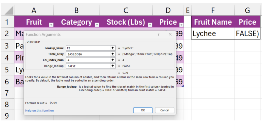
4. Fill in the fields step-by-step:

• Lookup_value: Click the selection box, then click cell F2.
• Table_array: Highlight cells A2:D6 on your sheet.
• Col_index_num: Type 4.
• Range_lookup: Type FALSE.

5. Look at the bottom of the Formula Builder pane—it will show you a preview of the result (in this case, $5.99).
6. Click OK or press Enter.

Performing VLOOKUP Between Different Sheets

In real-world business scenarios, your data isn’t always sitting neatly on the same worksheet. More often, your lookup tool is on Sheet 1, and your master inventory table is on Sheet 2.

To reference data on a different sheet, you must include the worksheet’s name followed by an exclamation mark (!) immediately before the table array.

Scenario 1: Sheet name has no spaces

If our master database is on a sheet named Inventory, the syntax is:

=VLOOKUP(A2, Inventory!$A$2:$D$6,4,FALSE)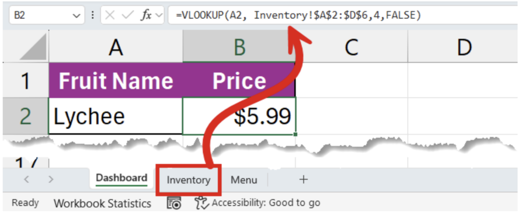

Scenario 2: Sheet name has spaces (Very Common!)

If your worksheet name has spaces (e.g., Master Inventory), you must wrap the sheet name in single quotes (‘), or Excel will throw an error:

=VLOOKUP(A2, 'Master Inventory'!$A$2:$D$6,4,FALSE)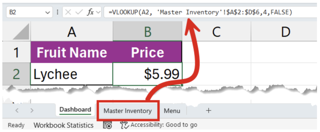

Troubleshooting Common VLOOKUP Errors

VLOOKUP is notoriously picky. If even one character is off, it will refuse to work. Here is how to diagnose and fix the most common spreadsheet roadblocks.

1. The Dreaded #N/A Error

This error means “Not Available.” Excel is telling you, “I looked everywhere in the first column, but I couldn’t find your lookup value.”

• The Fixes:

• Check for Typos: Check if your lookup value has spelling differences (e.g., searching for “Mangos” when the table says “Mango”).
• Clean Up Hidden Spaces: Extra spaces at the beginning or end of your text (like “Mango ” instead of “Mango”) are invisible to your eyes but completely different to Excel. Use the =TRIM() function to clean up messy datasets.
• Verify Column Order: Double-check that your lookup value is actually in the first column of your selected range.

Clean Up Your Dashboard with IFNA or IFERROR

Instead of letting ugly #N/A errors clutter your dashboard when a search is blank, wrap your VLOOKUP inside an IFNA function to display a clean, friendly message:

=IFNA(VLOOKUP(F2, $A$2:$D$6, 4, FALSE), "Fruit Not Found")

If there is no match, the cell will elegantly display “Fruit Not Found” instead of #N/A.

2. The #REF! Error

This means “Reference Error.” It occurs when your col_index_num is larger than the actual number of columns in your table_array.

• Example: Your table array is A2:D6 (4 columns wide), but you set your col_index_num to 5. Excel cannot look at Column 4 of a 3-column table!
• The Fix: Shrink your column index number or expand your table array range.

3. The #VALUE! Error

This happens if your col_index_num is less than 1 (e.g., 0 or a negative number), or if your formula contains broken formatting.

• The Fix: Ensure your column index is a positive integer greater than or equal to 1.

Power Moves: Using Wildcards for Partial Matches

What if you don’t know the exact name of the item you’re looking for? You can use wildcard characters in your lookup value to perform flexible, partial searches!

The Asterisk (*) – Matches any number of characters

If you want to search for an item and only know how it starts, use the asterisk.

• Lookup Value: “Mango*”
• Matches: “Mango”, “Mango Tommy”, “Mango Kent”, “Mangoes”.

Formula Example:

=VLOOKUP("Mango*", A2:D6, 4, FALSE)

The Question Mark (?) – Matches a single character

If you have product codes where only one character varies (like a size or region code), use the question mark.

• Lookup Value: “SKU-202?”
• Matches: “SKU-2024”, “SKU-202A”, “SKU-202B”.
• Does NOT match: “SKU-20210” (too many characters).

The Next Step: VLOOKUP vs. XLOOKUP

VLOOKUP has been the champion of data analysis for decades, and it is still vital to know because you will encounter it in millions of legacy spreadsheets globally.

However, if you are running newer versions of Excel (Excel 365 or Excel 2021+), you now have access to its modern successor: XLOOKUP.

XLOOKUP solves VLOOKUP’s biggest limitations:

• It can look left or right (no more ordering constraints).
• It defaults to an exact match (no more accidentally forgetting FALSE).
• It won’t break if you insert or delete columns in your database.

Make sure to master VLOOKUP first to ensure complete backward compatibility with older workbooks, and then check out our comprehensive guide to XLOOKUP to bring your skills into the modern era!

Take Your Excel Skills to the Next Level

Spreadsheet proficiency is one of the most consistently demanded skills in today’s job market. If you are ready to stop guessing and start building powerful, automated models, check out these highly recommended, practical training options designed to accelerate your workflow:

• Excel Shortcuts, Excel Tips, Excel Tricks – Excel Skills!
  Why Billy recommends it: If you want to stop hunting around menus and start flying through your workbooks at lightning speed, this is your pad. You’ll master the exact keyboard shortcuts, navigation strategies, and hidden tricks that seasoned professionals use to shave hours off their weekly tasks. No fluff—just pure execution speed.
• 7 Steps to Excel Success: Excel Skills and Power Tips
  Why Billy recommends it: This course is a beautifully structured roadmap to complete spreadsheet mastery. It breaks down the critical path from basic data architecture up to deploying advanced formulas and dynamic formatting. It’s perfect for anyone looking to build confidence, eliminate formula errors, and stand out in their career.
• Excel Tables: Organize, Analyze, and Present Your Data Like a Pro
  Why Billy recommends it: VLOOKUP’s absolute best friend is a properly formatted Excel Table! If you want to stop writing manual range coordinates (like $B$2:$E$6) and start using elegant, dynamic “Structured References” that expand automatically whenever you append new data rows, this training is an absolute game-changer. You will learn to easily filter, sort, format, and present massive datasets cleanly.

Now it’s your turn. Open up a fresh sheet, build a small data table, and write your first VLOOKUP formula. Once you get that first correct value returned without an error, I guarantee you’ll be hooked.

Keep on learning, and remember, don’t get mad…Get Skills!! 🤙