Excel Goal Seek – What it Does, and How to Use It

Excel is great for maintaining to-do lists, keeping a budget, tracking finances, and more. You can use it to organize tabular data sets, and perform a variety of calculations with that data. But what if you don’t know all the numbers involved in a calculation, or you want to test certain financial scenarios within the confines of a spreadsheet? That’s where Excel’s what-if analysis tools come in.

The goal seek function, part of Excel’s what-if analysis tool set, allows the user to use the desired result of a formula to find the possible input value necessary to achieve that result. Other commands in the what-if analysis tool set are the scenario manager and the ability to create data tables. This guide will focus on the goal seek command.

Udemy has numerous Excel classes aimed at beginners, as well as advanced Excel training for more experienced users.

Using Goal Seek

To get a better understanding of what the goal seek command actually does, create a spreadsheet that looks similar to this:

Step 1 – Set up a scenario

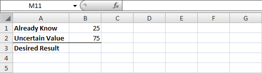
In cell A1, we have the text “Already Know,” used as a label for the value within our formula that we’re certain of. In this example, that value is 25, as seen in cell B1.

In cell A2, we have the text “Uncertain Value,” used as a label for the input value we want to determine. In the current equation, we have a value of 75, as seen in cell B2.

In cell A3, we have the text “Desired Result,” used as a label for the expected outcome of our equation.

Step 2 – Insert a formula

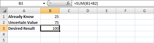
Next, select cell B3 and enter =SUM(B1+B2) into the formula bar, and press Enter. A value of 100 should appear in cell B3, the sum of cells B1 and B2. In other words, 25+75=100.

Step 3 – Select the Goal Seek command

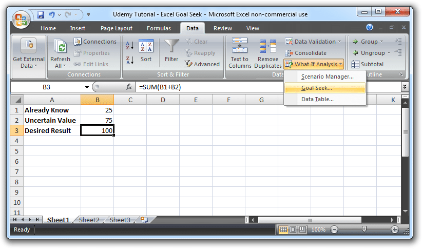
Next, navigate up to the Data tab in the ribbon menu. At the far right, there should be a group called Data Tools. Under the Data Validation and Consolidate options, you’ll find a drop-down menu for What-If Analysis. Select that, and from the menu, select Goal Seek.

Step 4 – Input the desired values

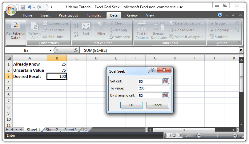
The goal seek function requires input for three options.

Set cell: Here, you need to input the name of the cell where the formula is located. For our example, that’s cell B3, which holds our formula =SUM(B1+B2).

To value: Here, you need to input the real desired value of our new equation, which the goal seek function will create. We’ll set it to 200. This means we want the sum of cells B1 and B2 to equal 200. However, we can only do that…

By changing cell: This one is very straightforward. The sum of cells B1 and B2 can only equal 200 by changing the value of one of our cells. In our example, we want to change cell B2, so we enter in B2. Then, click OK!

Step 5 – Success!

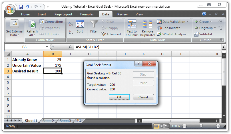
Once we hit OK, the computer finds that the only way to make the sum of cell B1 and cell B2 equal 200, when B1 remains 25 and B2 is an unknown value, is to change B2 to 175.

It’s basic math. It’s something you could solve in your head in a second. However, it can be applied to much more complicated mathematical scenarios and make for a more beneficial outcome. This example merely demonstrated its basic function.

Potential Sales Example

For a more applicable example, let’s say you run an online store where you sell hand-crafted necklaces at $18 each. You sell 35 of these a month for a monthly profit of $630. However, materials are getting more expensive, and after doing some calculations, you decide it’d be most convenient if you were to make $900 a month. But how much do you need to raise the price of your product to meet that goal?

Let’s create a basic spreadsheet:

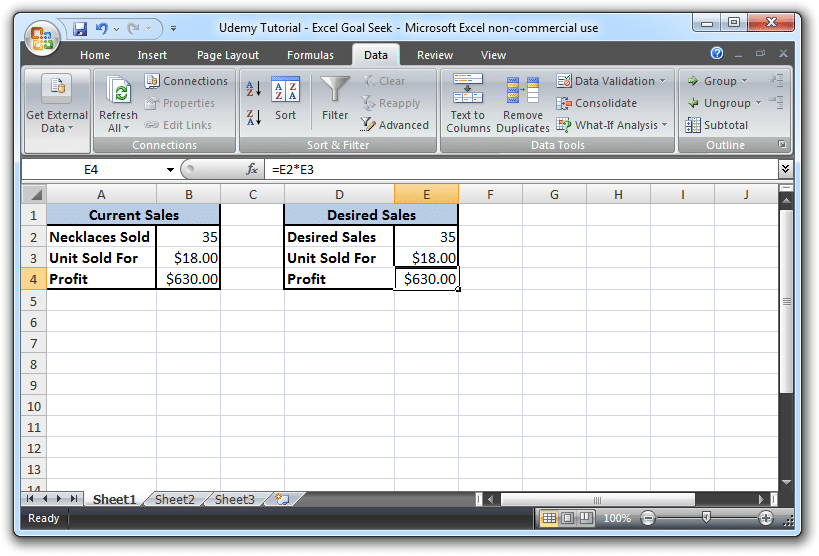
In our first table, we list our Current Sales information. In cell B2 we have 35, for number of necklaces sold per month, and in cell B3 we have $18.00, for the unit price per necklace. In cell B4, we enter the formula =E2*E3 to multiply the number of necklaces sold by the unit price, hit Enter, and come out with a profit of $630.00.

In our second table, we have the same information, but because this is our Desired Sales table, we’ll be changing some things up with the goal seek function.

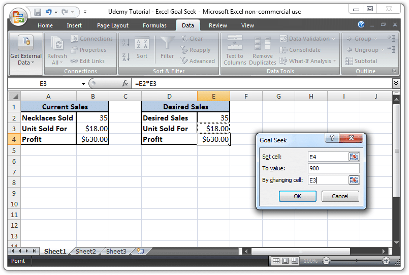
Set cell: We set E4, because that’s the cell where we want our newly calculated profit to go.

To value: We want the value of our new profit to be $900.00, so input 900 for this one.

By changing cell: We want to change the price of our product, not the amount of products sold, so input E3.

Goal seek will then change the value in cell E3 – where the price of our product is – into one that would, when multiplied by 35, equal 900.

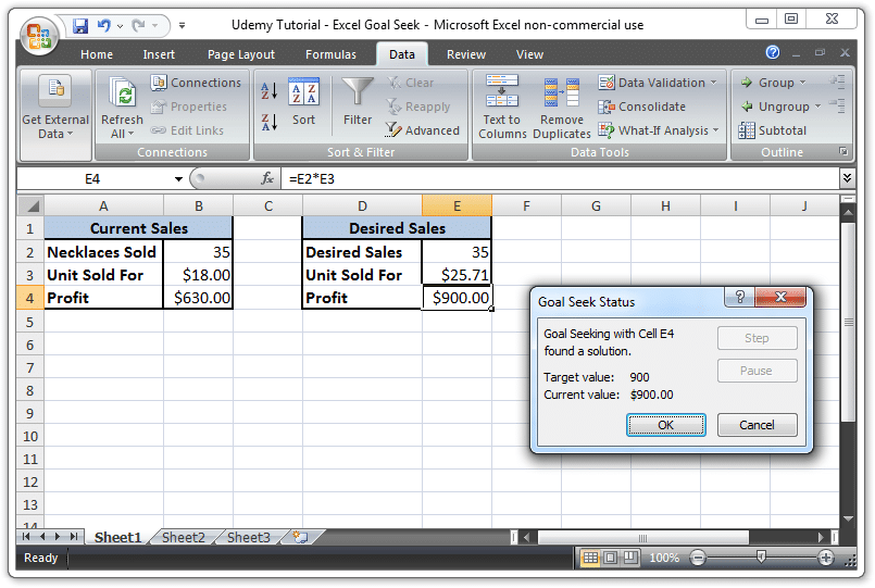
The goal seek function calculates that we will need to sell each necklace at $25.71 to make $900 a month. If we do the actual calculation here, we see that 25.71 x 35 = 899.85, while 26 x 35 = 910, meaning goal seek will round as close to the number as possible.

If we owned a store, we’d probably decide to round the number down ourselves, to 25 or 26, depending on circumstances. Nevertheless, goal seek has done its job.

What if the prices of materials haven’t changed, and we merely want to produce more items each month to turn out a bigger profit? We could use goal seek to figure this out just by inputting E2, instead of E3, into the “by changing cell” box.

At the end of the calculation, the what-if analysis tool will determine we need to sell 50 necklaces per month in order to make $900, exactly.

---

You can learn a lot more about Excel, and its various functions, with Udemy’s vast collection of Excel training courses.

You could take Excel Learning Made Easy, or a class on Basic and Advanced concepts in Excel, for users who want to embrace the full scope of the program’s applications.