Normal Distribution Example – Games of Chance

The news is full of accusations of the rigging of casino games and electronic games. When gamblers play slot machines over a long period of time, they expect to at least break even. When they do not, they may suspect the game is rigged. Some of us get lucky and win the jackpot during a short trip to Las Vegas, but this is not the normal experience of most players.  Introductory statistics can show us what the outcomes of a fairly played game of chance should look like.

A Toss of a Coin

After repeated play, the outcomes of fair games should follow normal distributions. Although we do not know the outcome of a game of chance in advance, we expect it to produce random variables that follow a bell curve shape distribution. The toss of a coin is an example.

The laws of probability dictate that if a coin is repeatedly tossed, over time, it will come up heads 50% of the time and tails 50% of the time. Likewise, if you play a fair game 1,000 times that does not depend on skill, you would expect to win 50% of the time. A slot machine is an example of such a game. The roll of the dice is another.

The peak of the bell curve is 50%, and the symmetrical sides represent the normal distribution of the random data around th average. The average of the random coin tosses is the peak of the bell curve, or mean, 50%. In a normal distribution, 50% of the values are less than the mean and 50% of the values are greater than the mean.

The bell curve is commonly used to evaluate school grades, ages of students, intelligent quotients (IQs), and many other variables. The mean IQ of the population is 100, and it has a standard deviation of 15. In classes, we take the average of all scores and call it the mean class average.

A Fair Roll of Dice

The outcome of a roll of dice is a well-known example of the bell curve. If a dice is rolled 100 times, the percentage of times a 1 turns up will be around 15% to 18%. If the dice is rolled 1,000 times, the percentage of times a 1 is rolled will fall within the 15% to 18% range, and will eventually converge to 16.7% (1/6).

In a fair roll of two dice, there are 36 possible combinations. The probability of rolling a 2 (1 + 1) is 2.8% (1/36).  The probability of rolling a 7 (with six possible combinations) is 16.7% (6/36).

This concept is also known as the law of averages. After many rolls, the average number of twos will be closer to the proportion of the outcome. The probabilities of the total set (all possible dice throws) must add up to one. Once we have determined the distribution of an event, we can figure out the probability that an event will happen in the future.

The Roulette Wheel and Standard Deviation

Let’s look at another example, the roulette wheel. George places his bet on the numbers 1 and 12. The probability of him winning is 12/38, and losing 26/38. Why? There are 38 slots on the roulette wheel. The chance that the ball will land on 1 is 2.63%. In gambling parlance, the odds are 37:1, or 1 chance in 38 that the ball will land on 1. The mean of the roulette game is 2.63%. All of George’s spin results are distributed randomly on either side of the mean.

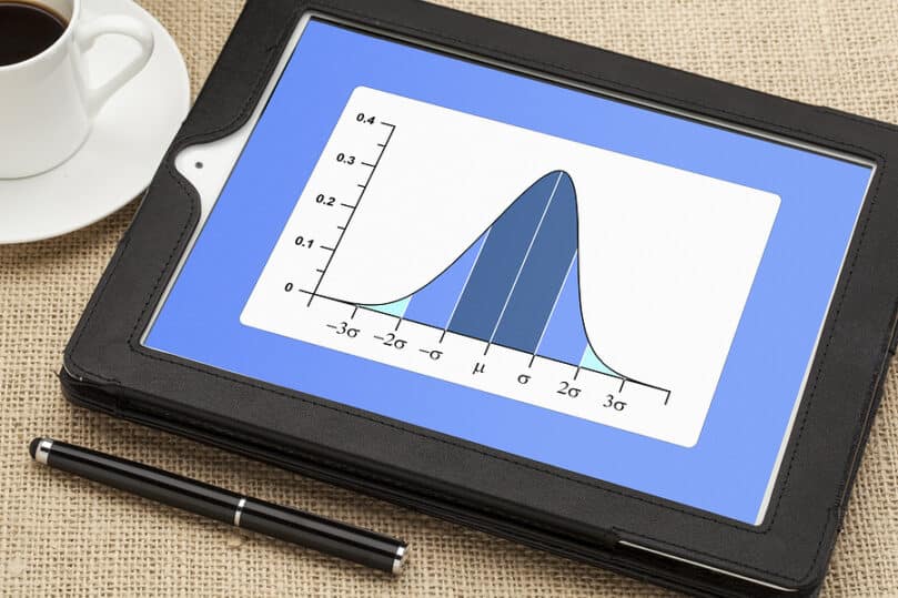
The bell curve is calculated by the mean and standard deviation. As shown, the mean is the average of the data, represented by the middle of the bell curve. The standard deviation is a measure of how spread out the numbers are. It is represented by the height and width of the bell curve. If the standard deviation is large, the data points are more spread out and the curve is shorter and wider. When the SD is small, the bell curve will be tall and narrow.

The total area of the bell curve is equal to 1 (100%)

About 68% of the area under the curve falls within 1 standard deviation.

About 95% of the area under the curve falls within 2 standard deviations.

About 99.7% of the area under the curve falls within 3 standard deviations.

Normal Distribution Calculator

Once we have confirmed that the roulette game follows a normal distribution, we can conclude that 95% of George’s spins will fall within two standard deviations on either side of the mean. Many statistical software packages are available to teach SPSS Essentials. SPSS allows you to plot and evaluate various outcomes. Through a chart called a Histogram, you can perform scenario analysis. Not all distributions are a bell curve, a normal distribution. The random data may be distributed to the right or skewed to the left. To experiment with different distributions data, use a normal distribution calculator.

In a normal distribution, the bell curve forms a symmetrical curve. Once we know the deviation of a distribution, we can forecast the probability that an outcome will fall within a range of the mean. Probability is shown in a range of 0 to 1. If an event has a probability of 0, it is not expected to occur. If an event has a probability of 1, it is likely to occur. Using the coin toss example, the probability that the coin toss will come up tails is 50%.

If game manufacturers are rigging games, as several lawsuits contend, the outcomes will not be fair, or normally distributed. To prove the case, the lawyers will need to calculate the probability of the expected outcomes of the rigged machines to prove that the results deviated from expected behavior. Law is just one area in which normal distribution applies. Since 17^th century French scientists discovered normal distribution while rolling dice, it has underpinned many disciplines. To master the practical application of statistics in your profession, enroll in The Workshop in Probability and Statistics or Quantifying the User Experience. Learning to use confidence intervals and hypothesis testing, and determine the size of errors and accuracy of estimates will help you establish the validity and reliability of the data you produce.